DeepSeek ’s latest moves have sent ripples through the AI community. Not only has it marked the beginning of a new era in artificial intelligence, but it has also made significant contributions to the open-source AI landscape. Their engineering techniques behind DeepSeek are truly impressive, and their reports are quite enjoyable. However, understanding their core ideas can be challenging and demands a substantial amount of effort.

At the forefront of this innovation is DeepSeek-R1, a model that built upon the foundation established by preceding projects such as DeepSeek Coder, Math, MoE, and notably, the DeepSeek-V3 model. While DeepSeek-R1 is the center of the DeepSeek’s frenzy, its success is rooted on these past works.

To help general readers navigate DeepSeek’s innovations more easily, I decided to write this post as a gentle introduction to their key components. I will begin by exploring the key ideas of V3 model, which serves as a cornerstone for DeepSeek-R1. I hope that this post will provide a clear and accessible explanation of their major contributions. Also, I strongly encourage you to read their reports :)

Contents

1. Multi-Head Latent Attention
   • Quick Review of Multi-Head Attention
   • Low-Rank Joint Compression
   • Efficient Computation Without Explicit Key & Value Computation
   • Decoupled RoPE
2. Mixture-of-Experts in DeepSeek
   • The Role of Shared Experts
3. Group Relative Policy Optimization
   • Proximal Policy Optimization
   • GRPO: PPO for DeepSeek
4. DeepSeek R1-Zero
5. Conclusion

Multi-Head Latent Attention

Quick Review of Multi-Head Attention

The query, key, and value in a standard multi-head attention (MHA) mechanism can be expressed as follows:

$$\begin{align*} \mathbf{q}_t &= W^{Q}\mathbf{h}_t\\ \mathbf{k}_t &= W^{K}\mathbf{h}_t\\ \mathbf{v}_t &= W^{V}\mathbf{h}_t \end{align*}$$

• $\mathbf{q}_t,\mathbf{k}_t,\mathbf{v}_t\in \mathbb{R}^{d_hn_h}$
• $\mathbf{h}_t\in \mathbb{R}^{d}$: Attention input of the $t$-th token at an layer.
• $d_h$: the attention head’s dimension
• $n_h$: the number of attention heads

During inference, all keys and values need to be cached to speed up computation. A cache requirement of MHA is roughly $2n_hd_hl$ elements per token (i.e., key, value for across all layers and heads). This heavy KV cache creates a major bottleneck, limiting the maximum batch size and sequence length during deployment.

Low-Rank Joint Compression

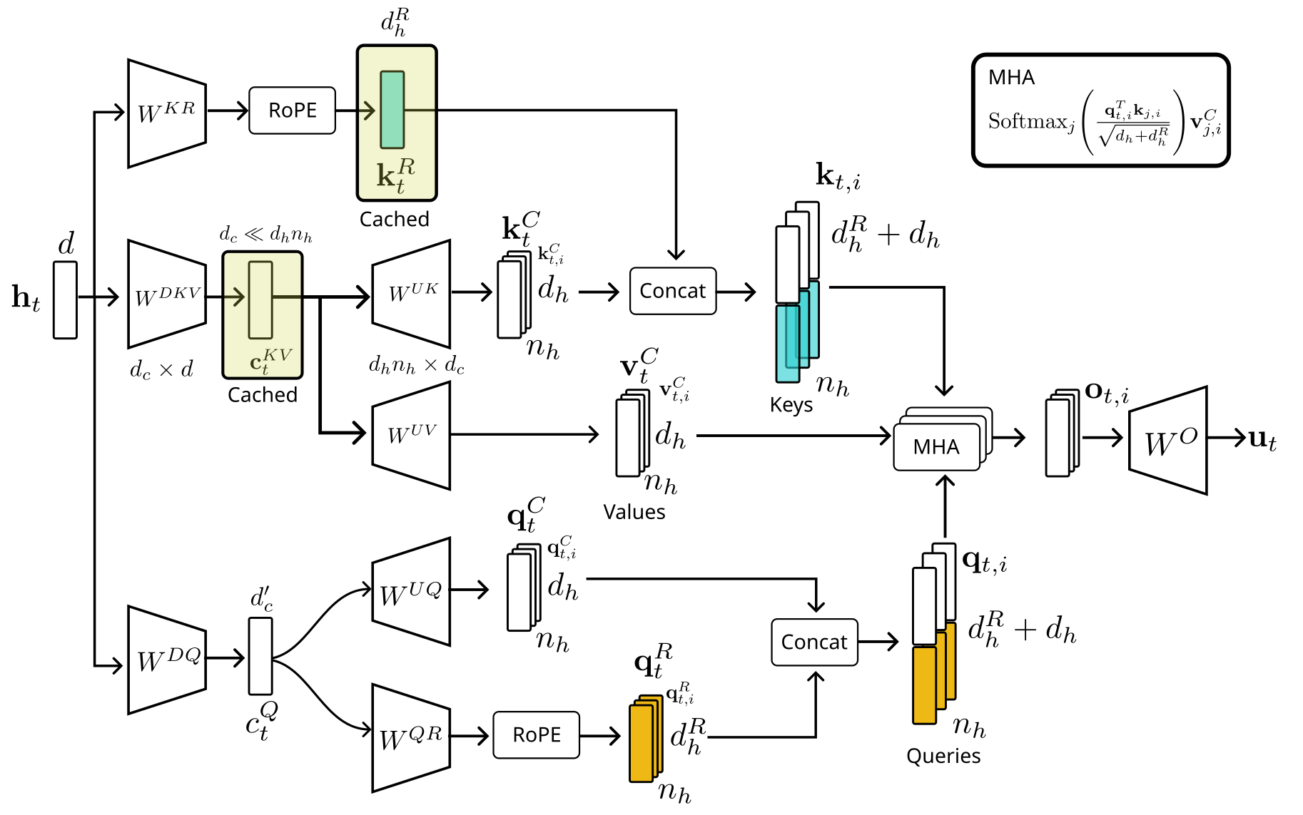
DeepSeek addresses this memory-intensive KV caching problem by introducing an alternative attention mechanism called Multi-Head Latent Attention (MLA). The core idea behind MLA is to compress keys and values into a low-dimensional latent space. Let’s break it down step by step:

$$\begin{align*} \mathbf{c}_t^{KV} &= W^{DKV}\mathbf{h}_t\\ [\mathbf{k}_{t,1}^C; \mathbf{k}_{t,2}^C; \dots ;\mathbf{k}_{t,n_h}^C] = \mathbf{k}_t^{C} &= W^{UK}\mathbf{c}_t^{KV}\\ \mathbf{k}_t^{R} &= \text{RoPE}(W^{KR}\mathbf{h}_t)\\ \mathbf{k}_{t,i} &= [\mathbf{k}_{t,i}^C;\mathbf{k}_t^{R}]\\ [\mathbf{v}_{t,1}^C; \mathbf{v}_{t,2}^C; \dots ;\mathbf{v}_{t,n_h}^C] = \mathbf{v}_t^{C} &= W^{UV}\mathbf{c}_t^{KV} \end{align*}$$

• The superscripts $D$ and $U$ denote the up- and down- projection, respectively.
• $\mathbf{c}_t^{KV}\in \mathbb{R}^{d_c}$ is the compressed latent vector for keys and values, where $d_c\ll d_hn_h$. Note that this is not a query vector.
• $W^{DKV}\in \mathbb{R}^{d_c\times d}$ is the down-projection matrix that generates the latent vector $\mathbf{c}_t^{KV}$.
• $W^{UK},W^{UV}\in \mathbb{R}^{d_hn_h\times d_c}$ are the up-projection matrices for keys and values, respectively. These operations help reconstruct the compressed information of $\mathbf{h}_t$.
• $W^{KR}\in \mathbb{R}^{d_h^R\times d}$ is the matrix responsible for generating the positional embedding vector. I will explain it soon.

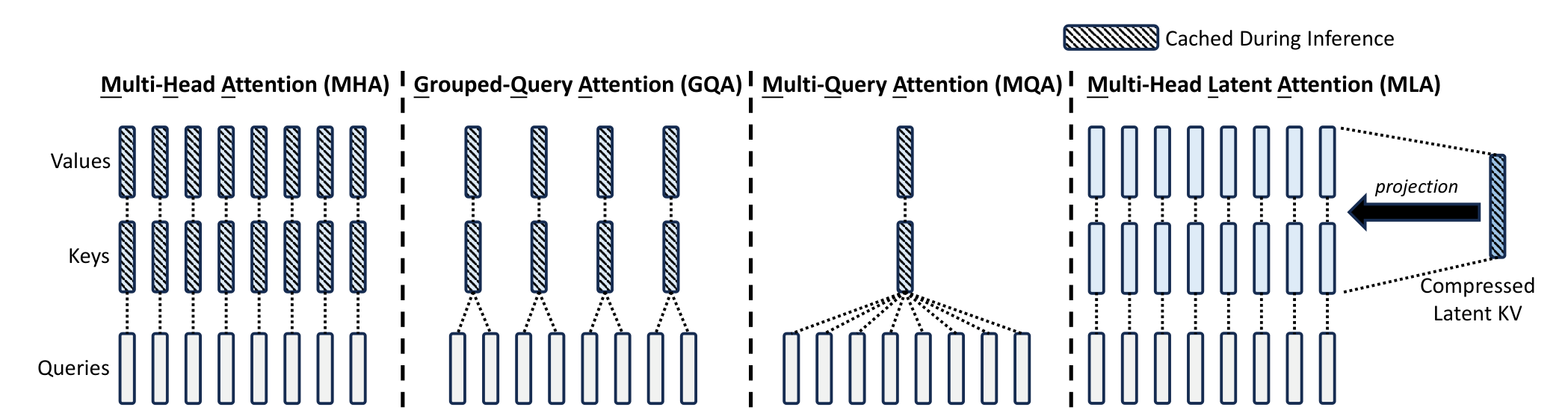
Unlike standard attention mechanisms like Grouped-Query Attention (GQA) or Multi-Query Attention (MQA), MLA only needs to cache the compressed vector $\mathbf{c}_t^{KV}$ during inference. MLA does not reduce the number of keys and values, allowing it to maintain the full representational power of self-attention while alleviating memory bottlenecks. The following figure provides an overview of KV-caching approaches in various attention mechanisms.

Efficient Computation Without Explicit Key and Value Computation

A key advantage of MLA is that it avoids explicit computation of the full-sized key and value matrices. Instead, attention scores can be computed as follows:

$$\begin{align*} q_t^Tk_t &= (W^{UQ}c_t^Q)^T(W^{UK}c_t^{KV})\\ &= (c_t^Q)^T(W^{UQT}W^{UK})c_t^{KV}, \end{align*}$$ where $W^{UQT}W^{UK}$ is a pre-computed matrix product of the two projection matrices. Similarly, for values: $$\begin{align*} o_{t,i} = \text{AttnScore}\cdot v_t^C. \end{align*}$$ The final output is given by $$\begin{align*} u_t &= W^O[o_{t,1}, \dots, o_{t,n_h}]\\ &= W^O[\text{AttnScore}\cdot (W^{UV}c_t^{KV})]\\ &= W^OW^{UV}[\text{AttnScore}\cdot (c_t^{KV})], \end{align*}$$ where $W^O\in \mathbb{R}^{d\times d_hn_h}$ is the output projection matrix.

Decoupled RoPE

A potential issue with MLA is how to incorporate positional embeddings (PE). While sinusoidal positional embeddings are a straightforward option, research has shown that Rotary Positional Embedding (RoPE) tends to provide better performance. However, applying RoPE in MLA poses a challenge: normally, RoPE modifies keys and values directly, which would require explicit computation of keys (i.e, $\mathbf{k}_t^{C}=W^{UK} c_t^{KV}$)—defeating the MLA’s efficiency.

DeepSeek circumvents this issue by introducing an explicit positional embedding vector $\mathbf{k}_t^{R}$, called decoupled RoPE. The PE vector is separately broadcasted across the keys. This allows MLA to benefit from RoPE without losing the efficiency gains of its compression scheme.

To further reduce activation memory during training, DeepSeek also compresses queries: $$\begin{align*} \mathbf{c}_t^{Q} &= W^{DQ}\mathbf{h}_t\\ [\mathbf{q}_{t,1}^C; \mathbf{q}_{t,2}^C; \dots ;\mathbf{q}_{t,n_h}^C] = \mathbf{q}_t^{C} &= W^{UQ}\mathbf{c}_t^{Q}\\ [\mathbf{q}_{t,1}^R; \mathbf{q}_{t,2}^R; \dots ;\mathbf{q}_{t,n_h}^R] = \mathbf{q}_t^{R} &= \text{RoPE}(W^{QR}\mathbf{c}_t^Q)\\ \mathbf{q}_{t,i} &= [\mathbf{q}_{t,i}^C;\mathbf{q}_{t,i}^{R}] \end{align*}$$

• $\mathbf{c}_t^{Q}\in \mathbb{R}^{d_c’}$ is the compressed latent vector for queries, where $d_c’\ll d_hn_h$
• $W^{DQ}\in \mathbb{R}^{d_c’\times d}$ and $W^{UQ}\in \mathbb{R}^{d_hn_h\times d_c’}$ are the down- and up- projection matrices for queries, respectively.
• $W^{QR}\in \mathbb{R}^{d_h^Rn_h\times d_c’}$ is the matrix for decoupled queries of RoPE.

Finally, the attention queries ($\mathbf{q}_{t,i}$), keys ($\mathbf{k}_{j,i}$), and values ($\mathbf{v}_{j,i}^C$) are combined to yield the final attention output $\mathbf{u}_t$: $$\begin{align*} \mathbf{o}_{t,i} &= \sum_{j=1}^t\text{Softmax}_j\Bigg( \frac{\mathbf{q}_{t,i}^T\mathbf{k}_{j,i}}{\sqrt{d_h+d_h^R}} \Bigg)\mathbf{v}_{j,i}^C,\\ \mathbf{u}_t &= W^O[\mathbf{o}_{t,1};\mathbf{o}_{t,2};\dots;\mathbf{o}_{t,n_h}]. \end{align*}$$

Mixture-of-Experts in DeepSeek

Traditional Mixture-of-Experts (MoE) models often suffer from two key issues:

• Knowledge Hybridity: Certain experts tend to cover a wide range of diverse knowledge rather than specializing in specific topics. This happens because input tokens are more frequently assigned to these experts than others, forcing them to handle vastly different types of knowledge.
• Knowledge Redundancy: Different experts often end up processing tokens that require overlapping knowledge. This redundancy limits expert specialization and efficiency.

If you are familiar with Principal Component Analysis (PCA), you may recognize that these issues in MoE are conceptually similar to the problems that PCA aims to address—eliminating redundancy and improving feature separation.

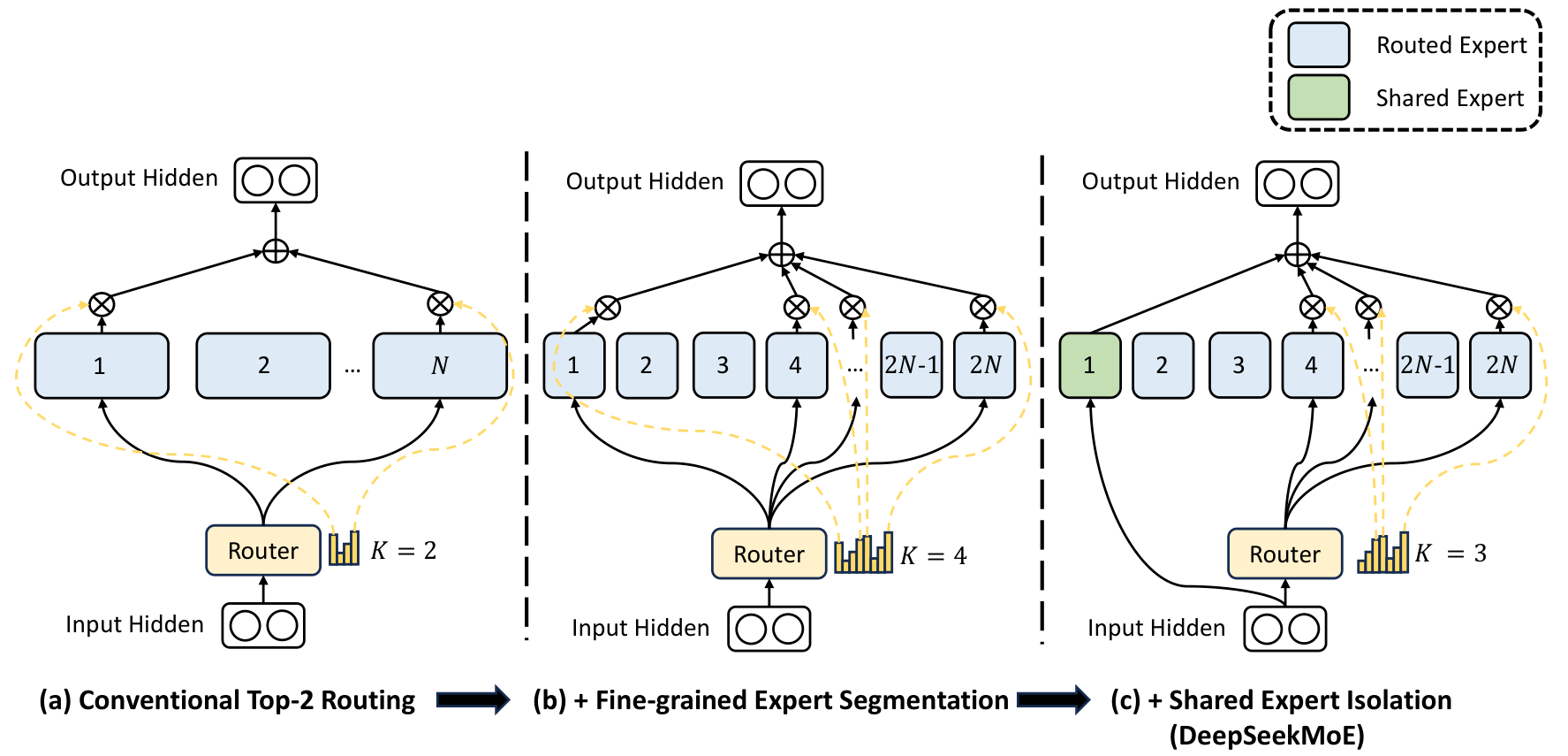
The above issues collectively hinder the effectiveness of expert in MoE architectures. To address them, DeepSeek introduces a novel approach that incorporates a dedicated expert for common knowledge, called a shared expert.

The following equation provides an overview of DeepSeek’s MoE architecture: $$\begin{align*} \mathbf{h}_t’ = \mathbf{u}_t+\sum^{N_s}_{i=1}FFN_i^{(s)}(\mathbf{u}_t)+\sum^{N_r}_{i=1}g_{i,t}FFN_i^{(r)}(\mathbf{u}_t), \end{align*}$$

• $\mathbf{u}_t$: FFN input of the $t$-th token.
• $\mathbf{h}_t’$ FFN output
• $N_s$ and $N_r$ are the number of shared experts and the routed experts, respectively.
• $FFN_i^{(s)}(\cdot)$ and $FFN_i^{(r)}(\cdot)$ are the $i$-th shared expert and the $i$-th routed expert, respectively.

The Role of Shared Experts

Unlike traditional MoE models, where all experts compete to process tokens, DeepSeek’s shared experts are always active. These experts are responsible for capturing and consolidating common knowledge across different input contexts. By concentrating general knowledge within shared experts, DeepSeek reduces redundancy among routed experts.

This separation of responsibilities allows routed experts to focus more effectively on specialized tasks, leading to better model efficiency and performance.

Group Relative Policy Optimization

DeepSeek introduces a reinforcement learning (RL) algorithm called Group Relative Policy Optimization (GRPO), a simple variant of Proximal Policy Optimization (PPO). If you have a basic understanding of RL and PPO, you’ll find GRPO quite straightforward. Let’s first review PPO.

Proximal Policy Optimization

PPO was proposed to address the instability of the vanilla policy gradient algorithm (i.e., REINFORCE algorithm). The core idea of PPO is to stabilize the policy update process by restricting the amount of update. The objective function of PPO is given by $$\begin{align*} \theta_{k+1} = \operatorname{argmax}_{\theta} \mathbb{E}_{s,a\sim \pi_{\theta_k}} [L(s, a, \theta_k, \theta)], \end{align*}$$ where $\theta_{k}$ is a parameter of a policy network at $k$-th step, $\theta$ is the current policy we want to update, and the $A$ is the advantage (\i.e., reward). Finally, the loss function $L$ is given by $$\begin{align*} L(s, a, \theta_k, \theta) = \min \left(\frac{\pi_{\theta}\left(a | s\right)}{\pi_{\theta_{\text {k}}}\left(a | s\right)} A^{\pi_{\theta_k}}(s,a), \text{ Clip}\Bigg(\frac{\pi_{\theta}\left(a | s\right)}{\pi_{\theta_{\text{k}}}\left(a | s\right)}, 1-\varepsilon, 1+\varepsilon\Bigg) A^{\pi_{\theta_k}}(s,a)\right). \end{align*}$$ Roughly, $\varepsilon$ is a hyperparameter which says how far away the new policy is allowed to go from the old one. A simpler expression of the above expression is $$\begin{align*} L(s, a, \theta_k, \theta) = \min \left(\frac{\pi_{\theta}\left(a | s\right)}{\pi_{\theta_{\text {k}}}\left(a | s\right)} A^{\pi_{\theta_k}}(s,a), g(\varepsilon, A^{\pi_{\theta_k}}(s,a)) \right), \end{align*}$$ where $$\begin{align*} g(\varepsilon,A) = \begin{cases} (1+\varepsilon)A & A\geq 0\\ (1-\varepsilon)A & A< 0. \end{cases} \end{align*}$$ There are two cases:

1. $A\geq 0$: The advantage for that state-action pair is positive, in which case its contribution to the objective reduces to $$\begin{align*} L(s, a, \theta_k, \theta) = \min \left(\frac{\pi_{\theta}\left(a | s\right)}{\pi_{\theta_{\text{k}}}\left(a | s\right)}, 1+\varepsilon \right) A^{\pi_{\theta_k}}(s,a). \end{align*}$$ Since the advantage is positive, the objective function increases if the action $a$ becomes likely under the policy (i.e., $\pi_{\theta}(a|s)$ increases). However, the $\min$ operator limits how much the objective can increase. Once $$\begin{align*} \pi_{\theta}(a|s) > (1+\epsilon) \pi_{\theta_k}(a|s), \end{align*}$$ the $\min$ ensures that the term is capped at $(1+\epsilon) A^{\pi_{\theta_k}}(s,a)$. This prevents the new policy from straying too far from the old policy.
2. $A<0$: The advantage for that state-action pair is negative, its contribution is given by $$\begin{align*} L(s, a, \theta_k, \theta) = \max \left(\frac{\pi_{\theta}\left(a | s\right)}{\pi_{\theta_{\text{k}}}\left(a | s\right)}, 1-\varepsilon \right) A^{\pi_{\theta_k}}(s,a). \end{align*}$$ Since the advantage is negative, the objective function increases if the action $a$ becomes less likely (i.e., $\pi_{\theta}(a|s)$ decreases). The $\max$ operator limits this increase. Once $$\begin{align*} \pi_{\theta}(a|s) < (1-\varepsilon) \pi_{\theta_k}(a|s), \end{align*}$$ the $\max$ caps the term at $(1-\varepsilon) A^{\pi_{\theta_k}}(s,a)$, again, ensuring that the new policy does not deviate too far from the old policy.

In sum, clipping serves as a regularizer by restricting the rewards to the policy, which change it dramatically with the hyperparameter $\varepsilon$ corresponds to how far away the new policy can go from the old while still profiting the objective.

GRPO: PPO for DeepSeek

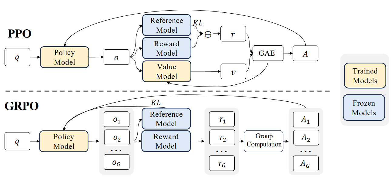
GRPO can be expressed as follows: $$\begin{align*} \mathcal{J} = \frac{1}{G}\sum_{i=1}^{G} \min \left(\frac{\pi_{\theta}\left(o_i | q\right)}{\pi_{\theta_{\text{k}}}\left(o_i | q\right)} A_i, \text{ Clip}\left(\frac{\pi_{\theta}\left(o_i | q\right)}{\pi_{\theta_{\text{k}}}\left(o_i | q\right)}, 1-\varepsilon, 1+\varepsilon\right) A_{i}\right) -\beta D_{KL}(\pi_{\theta}| \pi_{\text{ref}}). \end{align*}$$

• GRPO first samples a group of outputs ${o_1, o_2,\dots, o_G }$ from the old policy $\pi_{\theta_k}$
• Then it optimizes the policy model by maximizing the objective
• The KL-divergence is used to restrict the sudden change of policy.
• The advantage can be calculated by averaging and normalizing the rewards.
• Instead of using a value model explicitly, GRPO computes a value of the states (i.e., $o_i$) by averaging them. - Note that $A(s,a) = Q(s,a)-V(s)$
• $\pi_{\text{ref}}$ is the reference model, which is an initial SFT model.

DeepSeek-R1

DeepSeek-R1 is essentially a large language model fine-tuned using reinforcement learning. The process begins with training the DeepSeek-V3 model using the GRPO technique described earlier. Before applying RL, the model is pre-tuned with a small, carefully curated set of warm-up data designed to encourage logical outputs in a Chain-of-Thought (CoT) format. This preliminary step significantly improves training stability.

Interestingly, DeepSeek’s researchers first experimented with pure RL training—without any supervised signals—which led to the creation of DeepSeek-R1-Zero. Here are some observations from that experiment and my opinions.

DeepSeek R1-Zero

To train DeepSeek-R1-Zero, a rule-based reward signal was adopted. Two types of rewards are used:

• Accuracy rewards: The reward model evaluates whether the response is correct. For example, in math problems with deterministic results, the model is required to provide the final answer in a specified format, enabling reliable rule-based verification of correctness. Similarly, for LeetCode problems, a compiler can be used to generate feedback based on predefined test cases.
• Format rewards: In addition to the accuracy reward model, they employed a format reward model that enforces the model to put its thinking process between <think> and </think> tags.

Notably, DeepSeek-R1 does not rely on a neural reward model—likely because neural models may not consistently provide reliable rewards for training.

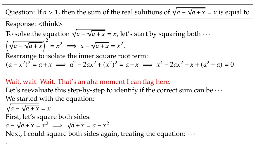
The team also reported an intriguing “aha moment” with DeepSeek-R1-Zero:

“DeepSeek-R1-Zero learns to allocate more thinking time to a problem by reevaluating its initial approach. This behavior is not only a testament to the model’s growing reasoning abilities but also a captivating example of how reinforcement learning can lead to unexpected and sophisticated outcomes.”

However, such behavior appears infrequently. More often, DeepSeek-R1-Zero tends to generate gibberish outputs, which may be attributed to the inherently unstable nature of RL training.

Conclusion

In this post, I’ve introduced some of the core ideas behind the DeepSeek-v3 and R1 models. While their deep learning techniques are undoubtedly interesting, I find their hardware-level engineering particularly more impressive. In my opinion, their success lies in these engineering achievements, and I look forward to exploring this aspect in a forthcoming post.