Latent Variable Modeling

Motivation of Latent Variable Modeling

Let’s say we want to classify some data. If we had access to a corresponding latent variable for each observation $ \mathbf{x}_i $, modeling would be more straightforward. To illustrate this, consider the challenge of finding the latent variable (i.e., the true class of $ \mathbf{x} $). It can be expressed like $ z^* = \argmax_{z} p(\mathbf{x} | z) $. It is hard to identify the true clusters without prior knowledge about them. For example, we can cluster like Fig. (b) or (c).

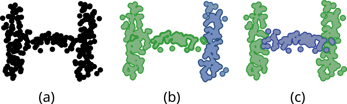
Consider modeling the complete data set $ p(\mathbf{x} | z) $ under the assumption that the observations are independent and identically distributed (i.i.d.). Based on the above Fig. (c), the joint distribution for a single observation $ (\mathbf{x}_i, \mathbf{z}_i) $ given the model parameters $ \boldsymbol{\theta} $ can be expressed:

\begin{align*} p(\mathbf{x}_i, \mathbf{z}_i | \boldsymbol{\theta}) = \begin{cases} p(\mathcal{C}_1) p(\mathbf{x}_i | \mathcal{C}_1) & \text{if } z_i = 0 \\ p(\mathcal{C}_2) p(\mathbf{x}_i | \mathcal{C}_2) & \text{if } z_i = 1 \\ p(\mathcal{C}_3) p(\mathbf{x}_i | \mathcal{C}_3) & \text{if } z_i = 2 \\ \end{cases} \end{align*} Given $ N $ observations, the joint distribution for the entire dataset $ { \mathbf{x}_1, \mathbf{x}_2, \ldots, \mathbf{x}_N } $ along with their corresponding latent variables $ { \mathbf{z}_1, \mathbf{z}_2, \ldots, \mathbf{z}_N } $ is:

\begin{align*} p(\mathbf{x}_1, \mathbf{x}_2, \dots, \mathbf{x}_N, \mathbf{z}_1, \mathbf{z}_2, \dots, \mathbf{z}_N | \boldsymbol{\theta}) = \prod_{n=1}^{N} \prod_{k=1}^{K} \pi_k^{z_{nk}} \mathcal{N}(\mathbf{x}_n | \boldsymbol{\mu}_k, \boldsymbol{\Sigma}_k)^{z_{nk}} \end{align*}

Here, $ \pi_k = p(\mathcal{C}_k) $ represents the prior probability of the $ k $-th component, and $ p(\mathbf{x}_n | \mathcal{C}_k) = \mathcal{N}(\mathbf{x}_n | \boldsymbol{\mu}_k, \boldsymbol{\Sigma}_k) $ denotes the Gaussian distribution associated with component $ \mathcal{C}_k $.

However, in practice, the latent variables $ \mathbf{z}_k $ are often not directly observable, which complicates the modeling process.

In the following sections, we present various methods for identifying and handling these latent variables to improve the classification and modeling of data.

K-Means Clustering

Suppose that we have a data set $\mathbf{X} = {\mathbf{x}_1,\dots, \mathbf{x}_n}$ consisting of $N$ observations of a random $D$-dimensional variable $\mathbf{x}\in \mathbb{R}^{D}$. Our goal is to partition the data into $K$ of clusters. Intuitively, a cluster can be thought as a group of data points whose inter-point distances are small compared with the distances to points outside of the cluster.

This notion can be formalized by introducing a set of $D$-dimensional vectors $\boldsymbol{\mu}_k$, which represents the centers of the clusters. Our goal is to find an assignment of data points to clusters, as well as a set of vectors ${\boldsymbol{\mu}_k}$. Objective function of $K$-means clustering (distortion measure) can be defined as follows: $$J = \sum_{n=1}^{N}\sum_{k=1}^{K}r_{nk}\lVert\boldsymbol{x}_n-\boldsymbol{\mu}_k\rVert^2$$ , where $r_{nk}\in{0,1}$ is a binary indicator variable which represents the membership of data $\mathbf{x}_n$. It can be expressed as follows: % The $r_{nk}$ can be optimized in a closed-form solution as follows: \begin{align*} r_{nk}=\begin{cases} 1 & \text{if } k=\argmin_{j} \lVert\boldsymbol{x}_n-\boldsymbol{\mu}_j\rVert^2\\ 0 & \text{otherwise} \end{cases} \end{align*} Our goal is to find values for the $\boldsymbol{\mu}_k$ and the $r_{nk}$ that minimize $J$.

We can minimize $J$ through an iterative procedure in which each iteration involves two successive steps corresponding to successive optimizations with respect to the $\boldsymbol{\mu}_k$ and the $r_{nk}$ First we choose some initial values for the $\boldsymbol{\mu}_k$. Then in the first phase we minimize $J$ with respect to the $r_{nk}$, keeping the $\boldsymbol{\mu}_k$ fixed. In the second phase we minimize $J$ with respect to the $\boldsymbol{\mu}_k$, keeping $r_{nk}$ fixed. This two-stage optimization is then repeated until convergence.

Now consider the optimization of the $\boldsymbol{\mu}_k$ with the $r_{nk}$ held fixed. The objective function $J$ is a quadratic function of $\boldsymbol{\mu}_k$, and it can be minimized by setting its derivative with respect to $\boldsymbol{\mu}_k$ to zero giving \begin{align*} 2\sum_{n=1}^{N}r_{nk}(\boldsymbol{x}_n-\boldsymbol{\mu}_k) = 0. \end{align*} We can arrange as \begin{align*} \boldsymbol{\mu}_k = \frac{\sum_n r_{nk}\boldsymbol{x}_n}{\sum_n r_{nk}}. \end{align*}

The denominator of $\boldsymbol{\mu}_k$ is equal to the number of points assigned to cluster $k$. The mean of cluster $k$ is essentially the same as the mean of data points $\mathbf{x}_n$ assigned to cluster $k$. For this reason, the procedure is known as the $K$-means clustering algorithm.

The two phases of re-assigning data points to clusters and re-computing the cluster means are repeated in turn until there is no further change in the assignments. These two phases reduce the value of the objective function $J$, so the convergence of the algorithm is assured. However, it may converge to a local rather than global minimum of $J$.

We can also sequentially update the $\mu_k$ as follows: \begin{align*} \mu_{k+1} = \mu_{k} + \eta(\mathbf{x}_k-\mu_{k}) \end{align*}

There are some properties to note:

• It is a hard clustering algorithm ($\leftrightarrow$ soft clustering)
• It is sensitive to the initialization of centroid.
• The number of clusters is uncertain.
• Sensitive to distance metrics (e.g., Euclidean?)

Gaussian Mixture Models

$K$-means clustering is a form of hard clustering, where each data point is assigned to exactly one cluster. However, in some cases, soft clustering—where data points can belong to multiple clusters with varying degrees of membership—provides a better model in practice. A Gaussian Mixture Model (GMM) assumes a linear superposition of Gaussian components, offering a richer class of density models than a single Gaussian distribution.

In essence, rather than assuming that all data points are generated by a single Gaussian distribution, we assume that the data is generated by a mixture of $ K $ different Gaussian distributions, where each Gaussian represents a different component in the mixture.

For a single sample, the Gaussian Mixture Model can be expressed as a weighted sum of these individual Gaussian distributions: \begin{align*} p(\mathbf{x}) &= \sum_\mathbf{z} p(\mathbf{z})p(\mathbf{x}|\mathbf{z}) \\ &= \sum_{k=1}^{K} \pi_k \mathcal{N}(\mathbf{x} | \boldsymbol{\mu}_k, \boldsymbol{\Sigma}_k) \end{align*} Here, $ \mathbf{x} $ is a data point, $ \pi_k $ represents the mixing coefficients, $ \mathcal{N}(\mathbf{x} | \boldsymbol{\mu}_k, \boldsymbol{\Sigma}_k) $ is a Gaussian distribution with mean $ \boldsymbol{\mu}_k $ and covariance $ \boldsymbol{\Sigma}_k $, and $ K $ is the number of Gaussian components.

A key quantity in GMMs is the conditional probability of $ \mathbf{z} $ given $ \mathbf{x} $, denoted as $ p(z_k = 1 | \mathbf{x}) $ or $ \gamma(z_k) $. This is also known as the responsibility or assignment probability, which represents the probability that a given data point $ \mathbf{x} $ belongs to component $ k $ of the mixture. Essentially, this can be thought of as the \textbf{classification result} for $ \mathbf{x} $.

This responsibility is updated using Bayes’ Theorem, and can be expressed as: \begin{align*} \gamma(z_k) \equiv p(z_k=1|\mathbf{x}) & \equiv \frac{p(z_k=1)p(\mathbf{x}|z_k=1)}{\sum_{j=1}^{K}p(z_j=1)p(\mathbf{x}|z_j=1)} \\ & = \frac{\pi_k\mathcal{N}(\mathbf{x}|\boldsymbol{\mu}_k, \boldsymbol{\Sigma}_k)}{\sum_{j=1}^{K} \pi_j\mathcal{N}(\mathbf{x}|\boldsymbol{\mu}_j, \boldsymbol{\Sigma}_j)} \end{align*}

In this expression, $ \pi_k $ is the prior probability (or mixing coefficient) for component $ k $, and $ \mathcal{N}(\mathbf{x} | \boldsymbol{\mu}_k, \boldsymbol{\Sigma}_k) $ is the likelihood of the data point $ \mathbf{x} $ under the Gaussian distribution corresponding to component $ k $. The denominator is a normalization factor that ensures the responsibilities sum to 1 across all components for a given data point.

This framework allows for a soft classification of data points, where each point is associated with a probability of belonging to each cluster, rather than being strictly assigned to a single cluster as in $K$-means.

Maximum Likelihood

Suppose we have a data set of observations $\mathbf{X}=\{ \mathbf{x}_1,\dots,\mathbf{x}_n \}^{T}\in\mathbb{R}^{N\times D}$ and we want to model the data distribution $p(\mathbf{X})$ using GMM. Assuming the data is independent and identically distributed (i.i.d.), the likelihood of the entire dataset can be expressed as: \begin{align*} p(\mathbf{X}|\boldsymbol{\pi},\boldsymbol{\mu},\boldsymbol{\Sigma}) = \prod_{n=1}^{N}\Bigg(\sum_{k=1}^{K}\pi_k\mathcal{N}(\mathbf{x}_n|\boldsymbol{\mu}_k, \boldsymbol{\Sigma}_k)\Bigg). \end{align*} To simplify the optimization process, we consider the log-likelihood function, which is given by: \begin{align*} \ln p(\mathbf{X}|\boldsymbol{\pi},\boldsymbol{\mu},\boldsymbol{\Sigma}) &= \sum_{n=1}^{N}\ln \Bigg(\sum_{k=1}^{K}\pi_k\mathcal{N}(\mathbf{x}_n|\boldsymbol{\mu}_k, \boldsymbol{\Sigma}_k)\Bigg) \end{align*} To solve the Maximum Likelihood Estimation (MLE) for Gaussian Mixture Models (GMMs), we typically consider the iterative Expectation-Maximization (EM) algorithm due to the non-convex nature of the problem. Before discussing how to maximize the likelihood, it is important to emphasize two significant issues that arise in GMMs: singularities and identifiability.

Singularity

A major challenge in applying the maximum likelihood framework to Gaussian Mixture Models is the presence of singularities. This problem arises because the likelihood function can become unbounded under certain conditions, leading to an ill-posed optimization problem.

For simplicity, consider a Gaussian mixture model where each component has a covariance matrix of the form $ \Sigma_k = \sigma^2_k I $, where $ I $ is the identity matrix. Suppose one of the mixture components, say the $ j $-th component, has its mean $ \boldsymbol{\mu}_j $ exactly equal to one of the data points $ \mathbf{x}_n $, so that $ \boldsymbol{\mu}_j = \mathbf{x}_n $ for some value of $ n $. The contribution of this data point to the likelihood function would then be: \begin{align*} \mathcal{N}(\mathbf{x}_n | \mathbf{x}_n, \sigma^2_j I) = \frac{1}{\sqrt{2\pi} \sigma_j} \cdot \exp^0 \end{align*} As $ \sigma_j $ approaches 0, this term goes to infinity, causing the log-likelihood function to also diverge to infinity. Therefore, maximizing the log-likelihood function becomes an ill-posed problem because such singularities can always be present. These singularities occur whenever one of the Gaussian components collapses onto a specific data point, leading to a covariance matrix with a determinant approaching zero. This issue did not arise with a single Gaussian distribution because the variance cannot be zero by definition.

Identifiability

Another issue in finding MLE solutions for GMMs is related to identifiability. For any given maximum likelihood solution, a GMM with $ K $ components has a total of $ K! $ equivalent solutions. This arises from the fact that the $ K! $ different ways of permuting the $ K $ sets of parameters (means, covariances, and mixing coefficients) yield the same likelihood.

In other words, for any point in the parameter space that represents a maximum likelihood solution, there are $ K! - 1 $ additional points that produce exactly the same probability distribution. This lack of identifiability means that the solution is not unique, complicating both the interpretation of the model and the optimization process.

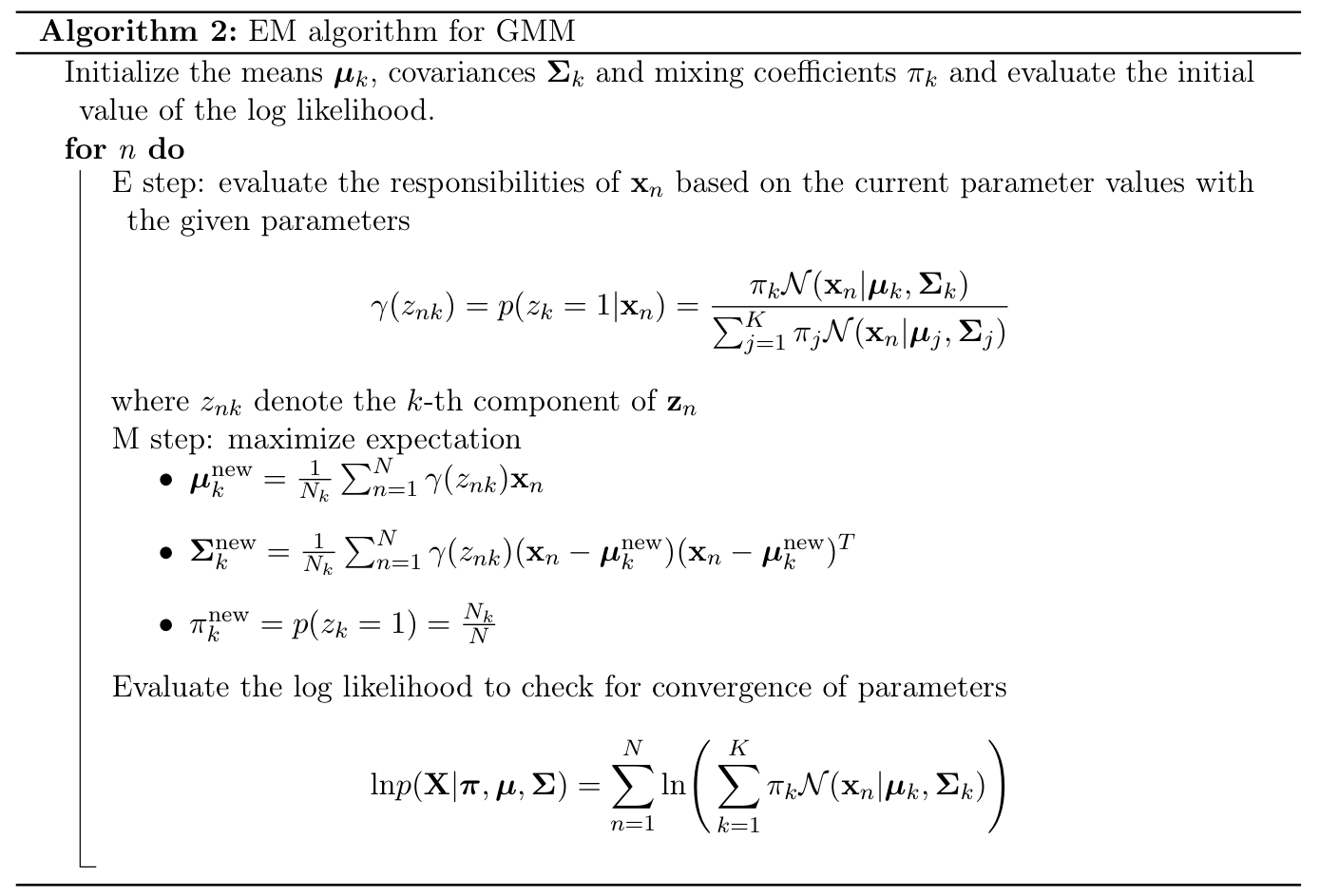
Expectation Maximization for GMM

The goal of the Expectation-Maximization (EM) algorithm is to find maximum likelihood solutions for models that involve latent variables.

• Suppose that directly optimizing the likelihood $p(\mathbf{X}|\boldsymbol{\theta})$ is difficult.
• However, it is easier to optimize the complete-data likelihood function $p(\mathbf{X}, \mathbf{Z}|\boldsymbol{\theta})$ as as discussed in the previous sections.
• In such cases, we can use the EM algorithm. EM algorithm is a general technique for finding maximum likelihood solutions in latent variable models.

Let’s begin by writing down the conditions that must be satisfied at a maximum of the likelihood function. By setting the derivatives of $\ln p(\mathbf{X}|\boldsymbol{\pi},\boldsymbol{\mu},\boldsymbol{\Sigma})$ with respect to the means $\boldsymbol{\mu}_k$ of the Gaussian components to zero, we obtain \begin{align*} 0 = -\sum_{n=1}^N\frac{\pi_k\mathcal{N}(\mathbf{x}|\boldsymbol{\mu}_k, \boldsymbol{\Sigma}_k)}{\sum_{j=1}^{K} \pi_j\mathcal{N}(\mathbf{x}|\boldsymbol{\mu}_j, \boldsymbol{\Sigma}_j)}\boldsymbol{\Sigma}_k(\mathbf{x}_n-\boldsymbol{\mu}_k) \end{align*} Multiplying by $\boldsymbol{\Sigma}_k^{-1}$ (which we assume to be non-singular) and rearranging we obtain \begin{align*} \boldsymbol{\mu}_k = \frac{1}{N_k}\sum_{n=1}^{N}\gamma(z_{nk})\mathbf{x}_n, \end{align*} where we have defined \begin{align*} N_k = \sum_{n=1}^{N}\gamma(z_{nk}). \end{align*} We can interpret $N_k$ as the effective number of points assigned to cluster $k$. We can obtain the MLE solutions for other variables similarly.

References:

• Christoper M. Bishop, Pattern Recognition and Machine Learning, 2006